Linear Mixed Models (LMMs)
A comprehensive explanation of Linear Mixed Models (LMMs), including their formulation and functionality, exploring how they handle hierarchical or correlated data structures through fixed and random effects to account for non-independence in datasets.


1.1. What is a Linear Mixed Model?
Linear mixed models (LMMs) can be thought of as a method for analyzing data that is non-independent, multilevel/hierarchical, longitudinal, or correlated.
1.2. Background
Linear mixed models are an extension of simple linear models to allow both fixed and random effects, and are particularly used when there is non independence in the data, such as arises from a hierarchical structure. For example, students could be sampled from within classrooms, or patients from within doctors.
When there are multiple levels, such as patients seen by the same doctor, the variability in the outcome can be thought of as being either within group or between group. Patient level observations are not independent, as within a given doctor patients are more similar. Units sampled at the highest level (in our example, doctors) are independent.

There are several methods to handle hierarchical data, each with its advantages and limitations. One straightforward approach is aggregation. For instance, if 10 patients are sampled from each doctor, instead of analyzing individual patient data—which are not independent— we could calculate the average for all patients under each doctor. This aggregated data would then be independent.
While analyzing aggregated data produces consistent estimates of effects and standard errors, it fails to fully utilize all available data, as patient-level information is reduced to a single average. For example, at the aggregated level, there would only be six data points, corresponding to the six doctors.
Another method for hierarchical data is analyzing one unit at a time. Using the same example, we could conduct six separate linear regressions, one for each doctor. Although this method is feasible, it has its limitations: the models operate independently, missing the opportunity to leverage data from other doctors, and resulting estimates can be "noisy" due to the limited data in each regression.
Linear mixed models (LMMs), also known as multilevel models, provide a balanced alternative between these two approaches. While individual regressions use detailed data but produce noisy estimates, and aggregation reduces noise but may overlook critical variations, LMMs strike a middle ground. They leverage data from all levels while accounting for the hierarchical structure inherent to the data.
Beyond correcting standard errors for non-independence, LMMs are valuable for examining differences in effects within and between groups. For example, consider a scatter plot showing the relationship between a predictor and an outcome for patients under six doctors. Within each doctor, the predictor-outcome relationship might be negative, but between doctors, the relationship could be positive. LMMs allow for the exploration of these nuanced effects, providing deeper insights into hierarchical data.
1.3. Random Effects
The foundation of mixed models lies in their ability to incorporate both fixed and random effects.
Fixed effects refer to parameters that remain constant across the population or study. For instance, we might assume there is a true regression line in the population, denoted as 𝛽, and our analysis provides an estimate of this value, \( \hat{\beta} \).
Random effects, on the other hand, are parameters treated as random variables. For example, we might assume that a random effect, \( \alpha_i \), follows a normal distribution with a mean of 𝜇 and a standard deviation of 𝜎, expressed mathematically as:
\[ \alpha_i \sim \mathcal{N}(\mu, \sigma) \]
This concept parallels linear regression, where the data points are considered random variables, while the parameters are fixed. However, in mixed models, both the data and certain parameters (the random effects) are treated as random variables, though at the highest level, overarching parameters - such as the population mean (𝜇) - remain fixed. This hierarchical structure allows mixed models to capture both population-level trends and group-specific variations effectively.
1.4. Theory of Linear Mixed Models (LMMs)
The general matrix definition of a LMM:
\[ \mathbf{y} = \boldsymbol{X\beta} + \boldsymbol{Zu} + \boldsymbol{\varepsilon} \]
Where:
To make the concept of mixed models more concrete, let’s explore an example using a simulated dataset. In this case, suppose N=8,114 patients were seen by J=407 doctors. The grouping variable is the doctor (j). The number of patients ( \( n_j \) ) seen by each doctor varies, ranging from as few as 2 to as many as 40, with an average of approximately 21 patients per doctor. The total number of patients is the sum of those seen across all doctors.
Our outcome variable (y) represents a continuous measure - mobility scores. Additionally, suppose we have six fixed-effect predictors:
- Age (in years),
- Married (0 = no, 1 = yes),
- Sex (0 = female, 1 = male),
- Red Blood Cell (RBC) count,
- White Blood Cell (WBC) count,
- A fixed intercept.
We also include a single random effect, the random intercept (q=1) for each of the J=407 doctors. For simplicity, we focus only on random intercepts, treating all other effects as fixed.
Random effects are necessary because we expect that mobility scores within each doctor’s group may be correlated. This could occur for several reasons:
- Specialization: Doctors may specialize in treating particular conditions (e.g., lung cancer patients with specific symptoms).
- Case Severity: Some doctors might handle more advanced cases, leading to more homogeneity within a doctor's group compared to between groups.
Random intercepts allow us to model this correlation within doctors’ groups, reflecting that patients treated by the same doctor tend to be more similar to one another than to patients treated by different doctors.
By stacking observations from all groups together, we account for all J=407 doctors in the model. Since q=1 for the random intercept model, the total number of random effect parameters is:
\[ qJ=(1)(407)=407 \]
The design matrix for random effects, Z, is large to represent explicitly. However, because we are only modeling random intercepts, Z has a simple and special structure. It serves as an indicator matrix, coding which doctor each patient belongs to. Specifically:
- Z consists of all 0s and 1s.
- Each column corresponds to one doctor (407 columns in this case).
- Each row corresponds to one patient (8,114 rows in total).
- If a patient belongs to the doctor represented by a particular column, the cell contains a 1; otherwise, it is 0.
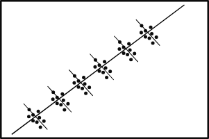
This structure makes Z a sparse matrix, meaning it contains mostly zeros. Sparse matrices are computationally efficient to store and process using specialized techniques.
The sparse nature of Z can be visualized in a graphical representation where:
- A dot (or a pixel) represents a non-zero entry (1), indicating a patient-doctor association.
- The line appears to "wiggle" because the number of patients per doctor varies, ranging from 2 to 40.
If we were to add a random slope (allowing the effect of one predictor, such as age, to vary across doctors), the structure of Z would change: the number of rows (corresponding to patients) would remain the same, but the number of columns would double because we would now have one column for the random intercept and another for the random slope for each doctor.
This doubling increases computational complexity, particularly when dealing with a large number of groups, as in this case with 407 doctors. Regardless of the number of random effects, Z remains sparse, but managing its size and complexity can become computationally burdensome as random effects increase.


If we estimated it, u would be a column vector, similar to β. However, in classical statistics, we do not actually estimate u. Instead, we nearly always assume that:
\[ \boldsymbol{u} \sim \mathcal{N}(\mathbf{0}, \mathbf{G}) \]
This statement can be understood as follows
- The random effects, denoted as 𝑢, are assumed to follow a normal distribution with a mean of zero and a variance-covariance matrix 𝐺.
- Here, 𝐺 represents the variance-covariance matrix of the random effects. The mean of the random effects is zero because random effects are modeled as deviations from the fixed effects. For instance, the fixed-effect intercept represents the overall mean, and the random intercepts represent deviations from this mean.
Estimation of Variance: Since the fixed effects (including the fixed intercept) are directly estimated, the random effects are deviations around these fixed effects. Therefore, the primary task when estimating random effects is to determine their variance, as their mean is fixed at zero.
- In our example, where there is only a random intercept, the matrix 𝐺 reduces to a 1×1 matrix, representing the variance of the random intercept. Mathematically:
\[ \mathbf{G}= [\sigma^{2}_{int}] \]
This single value \( {σ^2}_{int} \), is the variance of the random intercept.
Adding a Random Slope: If we extend the model to include both a random intercept and a random slope (allowing the effect of a predictor such as age to vary across groups), the structure of 𝐺 becomes more complex.
In this case:
- 𝐺 becomes a 2×2 matrix, with elements representing:
- The variance of the random intercept ( ( 𝜎^2_{int} ) ).
- The variance of the random slope ( ( 𝜎^2_{slope} ) ).
- The covariance between the random intercept and slope ( ( 𝜎_{int,slope} ) ).
Mathematically:
Because G is a variance-covariance matrix, we know that it should have certain properties. In particular, we know that it is square, symmetric, and positive semidefinite. We also know that this matrix has redundant elements. For a q×q matrix, there are q(q+1)/2 unique elements.
To simplify computation by removing redundant effects and ensure that the resulting estimate matrix is positive definite, rather than model G directly, we estimate θ, a triangular Cholesky factorization:
\[ \mathbf{G} = \mathbf{LDL^{T}} \]
θ is not always parameterized the same way, but we can generally think of it as representing the random effects. It is usually designed to contain non-redundant elements (unlike the variance covariance matrix) and to be parameterized in a way that yields more stable estimates than variances (such as taking the natural logarithm to ensure that the variances are positive). Regardless of the specifics, we can broadly say that:
\[ \mathbf{G} = \sigma(\boldsymbol{\theta}) \]
The final element in our model is the variance-covariance matrix of the residuals (ε) or the variance-covariance matrix of conditional distribution of \( (\mathbf{y} | \boldsymbol{\beta} ; \boldsymbol{u} = u) \). The common formulation for the residual covariance structure is:
\[ \mathbf{R} = \boldsymbol{I\sigma^2_{\varepsilon}} \]
where I is the identity matrix (diagonal matrix of 1s) and σ^2_ε is the residual variance. This structure assumes a homogeneous residual variance for all (conditional) observations and that they are (conditionally) independent.
Other structures can be assumed such as compound symmetry or autoregressive. The G terminology is common in SAS, and also leads to talking about G-side structures for the variance covariance matrix of random effects and R-side structures for the residual variance covariance matrix.
So the final fixed elements are y, X, Z, and ε. The final estimated elements are β^, θ^, and R^. The final model depends on the distribution assumed, but is generally of the form:
We could also frame our model in a two-leveled equation style: for the i-th patient for the j-th doctor. In this case we are working with variables that we subscript rather than vectors as before:
Substituting the level 2 equations into level 1, yields the mixed model specification. Here we grouped the fixed and random intercept parameters together to show that combined they give the estimated intercept for a particular doctor:
References
Fox, J. (2008). Applied Regression Analysis and Generalized Linear Models, 2nd ed. Sage Publications.
McCullagh, P, & Nelder, J. A. (1989). Generalized Linear Models, 2nd ed. Chapman & Hall/CRC Press.
Snijders, T. A. B. & Bosker, R. J. (2012). Multilevel Analysis, 2nd ed. Sage Publications.
Singer, J. D. & Willett, J. B. (2003). Applied Longitudinal Data Analysis: Modeling Change and Event Occurrence. Oxford University Press.
Pinheiro, J. & Bates, D. (2009). Mixed-Effects Models in S and S-Plus. 2nd printing. Springer.
Galecki, A. & Burzykowski, T. (2013). Linear Mixed-Effects Models Using R. Springer.
Skrondal, A. & Rabe-Hesketh, S. (2004). Generalized Latent Variable Modeling: Multilevel, longitudinal, and structural equation models. Chapman & Hall/CRC Press.
Gelman, A. & Hill, J. (2006). Data Analysis Using Regression and Multilevel/Hierarchical Models. Cambridge University Press.
Gelman, A., Carlin, J. B., Stern, H. S. & Rubin, D. B. (2003). Bayesian Data Analysis, 2nd ed. Chapman & Hall/CRC.
Good Resources for learning Regression Models and LMMs:


